Interpolation of Lidar Point Clouds

For representing terrain heights INSPIRE, which is aimed at creating an EU spatial data infrastructure, has developed specifications for digital terrain models (DTMs). DTMs are preferred as the main source for computing risks of flooding and other analytical tasks while their quality should be specified in terms of accuracy and resolution, i.e. grid size. Here, the author applies five interpolation methods to two airborne Lidar datasets both located in northwest Italy – one capturing a mountainous area and the other a flat urban area – and investigates the resulting accuracy for diverse grid sizes.

Interpolation Methods

The five interpolation methods used are: inverse distance weighting (IDW), natural neighbour (NN) and three variations on splines. In both the IDW and NN methods, heights of unknown points are calculated as a weighted average of known points in the vicinity. In IDW the influence of known points depends on a power of the distance to the unknown point. Other setting parameters are the number of known points and the size and shape of the search area. The power was set to 2, the radius to variable and the maximum number of points to 12. NN uses area derived from a Voronoi tessellation to define the weight. No parameters have to be specified. The third, fourth and fifth methods are based on splines. This approach is well suited for the creation of smoothly varying surfaces. The three variations on splines are: regularised (SpR), tension (SpT), and tension with barriers (SpTb). Breaklines may be included in SpTb by defining weight and number of points. For the regularised method, the weight defines the smoothness of the surface; the higher the weight, the smoother the surface. Typical values are 0, 0.001, 0.01, 0.1 and 0.5. In this study, 0.1 was used. In the tension method: the higher the weight, the coarser the surface. Typical values are 0, 1, 5, and 10. In this case, 0.1 was used. The more points, the smoother the surface will be at the expense of longer computation times. Here, the same number of points was used as for IDW, namely 12. Kriging has been excluded as the results would be similar to splines.

Test data and area

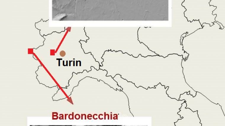
The test data, which was captured over two areas in Italy – Bardonecchia and Grugliasco (Figure 1) – has been acquired through airborne Lidar using the Leica Geosystems AL S50-II. This system employs multiple pulses in air (MPiA), has a maximum pulse rate of 150kHz and a scanning frequency of 90 lines per second while it records 4 returns, including first and last. The survey was originally aimed at creating orthoimagery at scale 1:5,000 and bare ground DTMs with height accuracy (combined systematic and random error) of 0.6m and a grid size of 5m. The actual survey was conducted with a pulse rate of 66.4kHz and scanning frequency of 21.4Hz while the intensities of the four returns were recorded. Points reflected on vegetation and buildings were removed using filters. Table 1 shows other key survey parameters. 

Table 1, Lidar survey specifications.

Although similar in size, the terrain characteristics of the two test areas differ significantly. Bardonecchia is located in the western Alps, close to the border with France, and covers an area of 39.20km² with altitudes varying from 1,230m to 2,200m. Grugliasco is an urban area located 10km west of Turin and covers 38.44km² with altitudes varying from 260m to 470m and is thus relatively flat. Over 12 million Lidar points were captured of the Bardonecchia site and nearly 11 million of the Grugliasco site, which results in – given the area – average densities of 1 point per 3.26m² and 1 point per 3.54m² respectively. Breaklines necessary for conducting interpolation by SpTb have been manually extracted from stereo imagery using a photogrammetric workstation.

Results

As the aim was to quantify how interpolation diminishes the accuracy with respect to the original Lidar points, around 1% of the Lidar points were randomly selected as check points. The other 99% were iteratively resampled to generate eight subsets with subsequent lower densities (Table 2). Each subset was interpolated with the five methods described above at three grid sizes: 5 x 5m, 10 x 10m and 20 x 20m. Next each grid height was compared with the height at the check point. To determine the height at the exact corresponding location, bilinear interpolation was applied using four surrounding check points. The root mean square error (RMSE) was computed using Esri ArcGis 10.1 and Python scripting. Residuals and statistical analyses were executed using the free software environment for statistical computing and graphics of the R project (http://www.r-project.org/).

Table 2, Eight subsets created by iteratively resampling to courser densities.

The resulting 24 RMSEs per method for Bardonecchia are shown in Figure 2 and for Grugliasco in Figure 3. Note that 0 on the horizontal axis indicates the original point density. The RMSEs of Grugliasco (flat urban area) are an order of magnitude of 3 to 4 better than those of Bardonecchia. IDW and NN succeeds in generating the grids of all 8 subsets. Splines are unable to cope with the denser datasets up to 1 point per 10m² and even produce peaks. The saw-tooth shapes of the graphs clearly indicate that – as could be expected – accuracy decreases as point density decreases, i.e. RMSE becomes larger, with IDW being most affected (pink lines). With increasing grid size, accuracy decreases rapidly for all methods and this effect is more severe for the urban area (Grugliasco) than for the mountainous area (Bardonecchia).

Acknowledgements

Thanks are due to Gianni Siletto for providing the airborne Lidar data.

Further Reading

Bater C. W., Coops N. C. (2009) Evaluating error associated with Lidar-derived DEM interpolation, Computers & Geosciences, 35:2, pp. 289-300.

Godone D., Garnero G. (2013) The role of morphometric parameters in digital terrain models interpolation accuracy: A case study, European Journal of Remote Sensing, 46:1, pp. 198-214.

Guarnieri A., Vettore A., Pirotti F., Menenti M., Marani M. (2009) Retrieval of small-relief marsh morphology from terrestrial laser scanner, optimal spatial filtering, and laser return intensity, Geomorphology,113: 1–2, pp. 12-20.

Guo Q., Li W., Yu H., Alvarez O. (2010) Effects of topographic variability and Lidar sampling density on several DEM interpolation methods, Photogrammetric Engineering & Remote Sensing, 76:6, pp. 701 – 712.

Lemmens, M. (2014) Point Clouds (1) – The functionalities of processing software, GIM International, 28:6, pp. 16-21.

Gabriele Garnero is a professor of geomatics at the University of Turin and of planning sciences at the Polytechnic of Turin, Italy. His research interests include applications of GNSS, photogrammetry and remote sensing; architectural surveys; digital cartography, GIS and cadastral applications.

gabriele.garnero@unito.it