Integrating UAV-based Lidar and photogrammetry

A UAV project in Germany has integrated photogrammetric bundle block adjustment with direct georeferencing of Lidar point clouds to considerably improve the respective accuracy.

Recent unmanned aerial vehicle (UAV or ‘drone’) platforms jointly collect imagery and Lidar data. Their combined evaluation potentially generates 3D point clouds at accuracies and resolutions of some millimetres, so far limited to terrestrial data capture. This article outlines a project that integrates photogrammetric bundle block adjustment with direct georeferencing of Lidar point clouds to improve the respective accuracy by an order of magnitude. Further benefits of combined processing result from adding Lidar range measurement to multi-view-stereo (MVS) image matching during the generation of high-precision dense 3D point clouds.

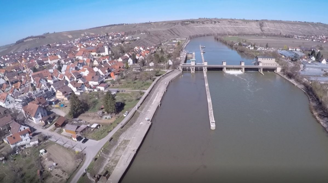
The project was aimed at the area-covering monitoring of potential subsidence of about 10 mm/year by a repeated collection of very accurate and dense 3D point clouds. The considerable size of the test site in Hessigheim, Germany, prevents terrestrial data capture. As visible in Figure 1, the site consists of built-up areas, regions of agricultural use and a ship lock as the structure of special interest.

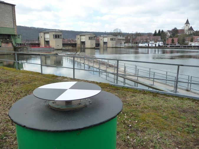
For traditional monitoring, a network of several pillars was established in the vicinity of the lock. As depicted in Figure 2, photogrammetric targets signalized the pillars to make them available as check and control points for georeferencing. For UAV data collection, a RIEGL RiCopter octocopter was used equipped with a RIEGL VUX-1LR Lidar sensor and two Sony Alpha 6000 oblique cameras. With a nominal flying altitude of 50m above ground level, a strip distance of 35m and a scanner field of view (FoV) of 70°, the system captured 300-400 points/m² per strip and 800 points/m² for the entire flight block due to the nominal side overlap of 50%. The flight mission parameters resulted in a laser footprint diameter on the ground of less than 3cm with a point distance of 5cm. The ranging noise of the scanner is 5mm. The trajectory of the platform was measured by an APX-20 UAV GNSS/IMU system to enable direct georeferencing. The two Sony Alpha 6000 oblique cameras mounted on the RiCopter platform have a FoV of 74° each. Mounted at a sideways-looking angle of ±35°, they captured imagery at a ground sampling distance (GSD) of 1.5-3cm with 24 megapixels each.

Lidar strip adjustment and automatic aerial triangulation

After direct georeferencing, a typical Lidar workflow includes a strip adjustment to minimize differences between overlapping strips. This step improves georeferencing by estimating the scanner’s mounting calibration as well as correction parameters for the GNSS/IMU trajectory solution. Typically, a constant offset (Δx, Δy, Δz, Δroll, Δpitch, Δyaw) is estimated for each strip. Alternatively, time-dependent corrections for each of these six parameters can be modelled by splines.

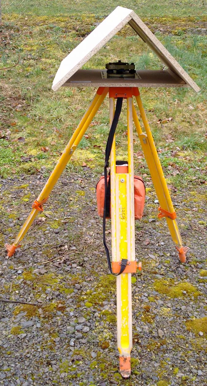
Figure 3 exemplarily depicts a Lidar ground control plane used for absolute georeferencing. Each signal features two roof-like oriented planes at a size of 40cm × 80cm with known position and orientation. The evaluation of this project’s Lidar strip adjustment additionally applies the signallized pillars depicted in Figure 2. These photogrammetric targets provide elevation differences to the georeferenced point cloud at 33 targets. In the investigations, these differences resulted in an RMS accuracy of 5.2cm. To enable georeferencing of the Sony Alpha oblique image block by automatic aerial triangulation (AAT), six of the photogrammetric targets were selected as ground control points (GCPs). The remaining 27 targets provided differences at independent check points (CPs) ranging between 5.2cm (max.) and 1.2cm (min.) with an RMS of 2.5cm.

Thus, neither the Lidar strip adjustment nor bundle block adjustment yield the required 3D object point accuracy during an independent evaluation of the different sensor data. However, accuracy improves significantly if both steps are integrated by so-called hybrid georeferencing (Glira 2019).

Hybrid georeferencing of airborne Lidar and imagery

Figure 4 depicts a section of the project’s Lidar points, colour-coded by the intensity value. The overlaid white points represent tie points from the bundle block adjustment of the Sony Alpha imagery. Usually, this step estimates the respective camera parameters from corresponding pixel coordinates of overlapping images. The object coordinates of these tie points are just a by-product.

In contrast, hybrid georeferencing applies these tie point coordinates to minimize their differences to the corresponding Lidar points. This process estimates time-dependent corrections of the flight trajectory similar to traditional Lidar strip adjustment. Within this step, tie point coordinates add geometric constraints from AAT. This provides considerable constraints from the image block to correct the Lidar scan geometry. This is especially helpful if both sensors are flown on the same platform and thus share the same trajectory. Hybrid georeferencing additionally opens up information on ground control points used during bundle block adjustment. Thus, georeferencing of Lidar data no longer requires dedicated Lidar control planes. Instead, all the required check point and control point information is available from the standard photogrammetric targets, which is of high practical relevance.

The authors applied a flexible spline as a powerful model for trajectory correction. This flexibility can potentially result in systematic deformations if applied during standard strip adjustment. In contrast, integrating information from stable 2D image frames as oriented during bundle block adjustment reliably avoids such negative effects. Figure 5 depicts the result of the hybrid approach from the OPALS software used. The six GCPs marked by the red circles and the remaining 27 targets used as CPs coincide with the AAT already discussed. For hybrid georeferencing, the elevation differences are -1.5cm minimum, 0.7cm maximum and -0.4cm mean. The corresponding standard deviation of 0.6cm clearly indicates that sub-centimetre accuracy is now feasible.

Combined point clouds from Lidar and multi-view stereo

Photogrammetric tie points as depicted in Figure 4 are just a by-product of bundle block adjustment, since dense 3D point clouds are provided by MVS in the subsequent step. In principle, the geometric accuracy of MVS point clouds directly corresponds to the GSD and thus the scale of the respective imagery. This allows 3D data capture even in the sub-centimetre range for suitable image resolutions. However, stereo image matching presumes the visibility of object points in at least two images. This can be an issue for very complex 3D structures. In contrast, the polar measurement principle of Lidar sensors is advantageous whenever the object appearance changes rapidly when seen from different positions. This holds true for semi-transparent objects like vegetation or crane bars (see Figure 4), for objects in motion like vehicles and pedestrians, or in very narrow urban canyons as well as on construction sites. Another advantage of Lidar is the potential to measure multiple responses of the reflected signals, which enables vegetation penetration. On the other hand, adding image texture to Lidar point clouds is advantageous for both visualization and interpretation. In combination with the high-resolution capability of MVS, this supports the argument to properly integrate Lidar and MVS during 3D point cloud generation.

 

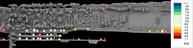
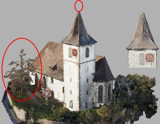
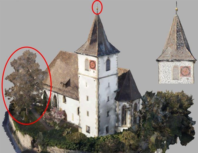
Figure 6 shows a 3D textured mesh generated from the Sony Alpha images by the MVS pipeline realized in the SURE software from nFrames. As can be seen in Figure 7, much more geometric detail is available, e.g. on the top of the church and in vegetation after Lidar data is integrated. Face count typically adapts to the geometric complexity, which is also visible for the small section of the church tower. As an example, Figure 6 consists of approximately 325,000 faces, while Figure 7 features 372,000 triangles.

 

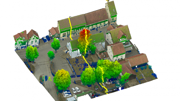
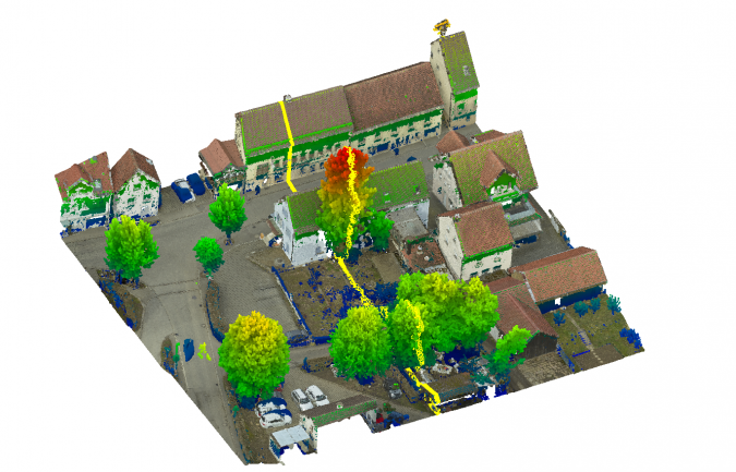
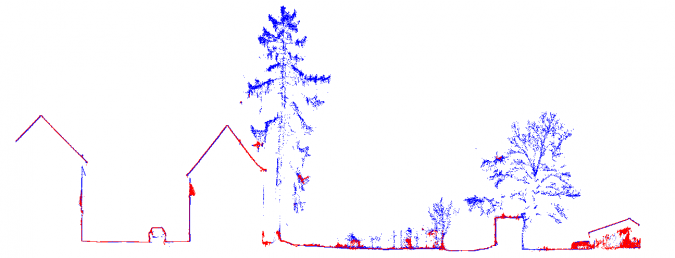
Figures 8 and 9 demonstrate the complementary characteristics of Lidar and MVS for 3D points at another part of the test site. Figure 8 depicts the RGB-coloured points generated by MVS; the overlaid Lidar data is colour-coded according to the respective elevation. Lastly, the yellow line represents the profile used to extract the points depicted in Figure 9. The discrepancies between the point clouds from MVS (red) and Lidar (blue) are especially evident at trees, where Lidar allows the detection of multiple returns along a single laser ray path.

 

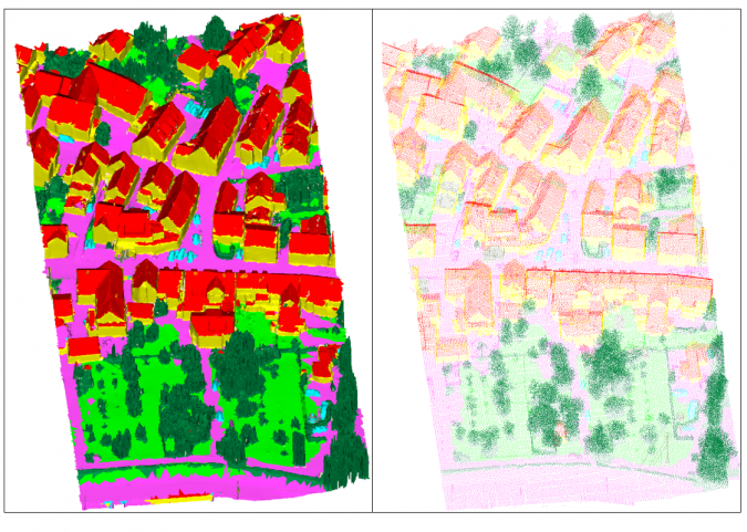
Whereas point clouds as shown in Figures 8 and 9 are an unordered set of points, meshes as depicted in Figures 6 and 7 are graphs consisting of vertices, edges and faces that provide explicit adjacency information. The main differences between meshes and point clouds are the availability of high-resolution texture and the reduced number of entities. This is especially useful for subsequent automatic interpretation. Generally, many (Lidar) points can be associated with a face. The authors utilized this many-to-one relationship to enhance faces with median Lidar features derived from the respective associated points. This enabled them to integrate inherent information from both sensors in the mesh representation in order to achieve the best possible semantic segmentation. Figure 10 shows the labelled mesh as predicted by a PointNet++ classifier (left) and the labels transferred to the dense Lidar point cloud (right), subsampled by factor 20 for visualization. The following class colour code is used: facade (yellow), roof (red), impervious surface (magenta), green space (light green), mid and high vegetation (dark green), vehicle (cyan), chimney/antenna (orange) and clutter (gray).

 

The forwarding was accomplished easily by re-using the many-to-one relationship between Lidar points and faces. Thereby, the semantic segmentation of the Lidar point cloud uses features that have originally only been available for the mesh, e.g. texture. Hence, the semantic mesh segmentation uses inherent features from both representations, which is another benefit of joint image and Lidar processing.

 

Conclusion

This article presents a workflow for hybrid georeferencing, enhancement and classification of ultra-high-resolution UAV Lidar and image point clouds. Compared to a separate evaluation, the hybrid orientation improves accuracies from 5cm to less than 1cm. Furthermore, Lidar control planes become obsolete, thus considerably reducing the effort for providing control information on the ground. The authors expect a further improvement by replacing the current cameras mounted on the RIEGL RiCopter with a high-quality Phase One iXM system to acquire imagery of better radiometry at higher resolution. This will further support the generation and analysis of high-quality point clouds and thus enable UAV-based data capture for very challenging applications.

Acknowledgements

Parts of the presented research were funded within a project granted by the German Federal Institute of Hydrology (BfG) in Koblenz. Thanks go to Gottfried Mandlburger, Wilfried Karel (TU Wien) and Philipp Glira (AIT) for their support and adaption of the OPALS software during hybrid georeferencing. The support of Tobias Hauck from nFrames during joint work with SURE is also acknowledged.