Lidar Crop Classification with Data Fusion and Machine Learning

A recent study created crop type maps using Lidar, Sentinel-2 and aerial data along with several machine learning classification algorithms for differentiating four crop types in an intensively cultivated area. Crop type maps are frequently generated using remotely sensed data acquired by sensors mounted on satellites, manned aircraft or unmanned aerial vehicles (UAVs or ‘drones’), the most popular being multispectral sensors mounted on satellites. Aerial multispectral sensors are more frequently employed where imagery with very high spatial resolution is required. However, the use of Lidar data for crop type mapping is still uncommon.

Lidar data is becoming ever-more widely available as more aerial surveys are conducted, UAV-Lidar sensors are becoming more prevalent and Earth observation satellites are being fitted with Lidar sensors. Crop type mapping can benefit from these new sources of Lidar data, especially when combined with high-resolution, multispectral and multi-temporal optical imagery such as that provided by the Sentinel-2 constellation. This combination of Lidar data and optical imagery can bode well for the agricultural sector when used to produce more accurate crop type classifications.

Lidar is commonly used in remote sensing to collect surface height information by either using the 3D point cloud or by interpolating a digital surface model (DSM) or digital terrain model (DTM). From the DSM and DTM, a normalized DSM (nDSM), or canopy height model (CHM), can be derived by subtracting the DTM from the DSM. Photogrammetry methods can also be used to create a DSM. However, Lidar can penetrate vegetation canopies and obtain accurate height information of the terrain below and in turn be used to create a DTM and subsequently an nDSM. Besides the height information, Lidar also provides returned intensity information which can be used to differentiate between different land covers. For instance, scanning water results in low-intensity returns, while the intensity of returns from vegetation is high.

Study area in South Africa

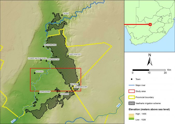
In recent research, the Vaalharts irrigation scheme located in the Northern Cape Province of South Africa was used for the study area (Figure 1). The study area was selected due to the availability of Lidar data. The irrigation scheme is situated at the confluence of the Harts and Vaal rivers and contains various types of land cover, including indigenous vegetation, built-up areas, bare ground, water and crops including cotton, maize, wheat, barley, lucerne, groundnuts, canola and pecan nuts, all of which are grown on a crop rotation basis.

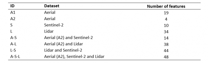
The datasets

Three datasets were used, namely Lidar data, aerial imagery and satellite imagery. The Lidar and aerial imagery were captured by Land Resources International for the Northern Cape Department of Agriculture, Land Reform and Rural Development. The Lidar data was collected between 19 and 29 February 2016 with a Leica ALS50-II Lidar sensor at an altitude of 4,500ft, resulting in an average point spacing of 0.7m and an average point density of 2.04m². The aerial imagery was collected between 22 February and 18 March 2016 using a PhaseOne iXA multispectral sensor at an altitude of 7,500ft and consisted of four bands, namely blue, green, red and near-infrared (NIR). The aerial imagery had a ground sampling distance (GSD) of 0.1 m for the blue, green and red bands and a GSD of 0.5m for the NIR band. The Sentinel-2 imagery was collected on 10 February 2016 and was selected due to the lack of cloud cover and the temporal match to the Lidar data and aerial imagery. The four 10m-resolution bands and the six 20m-resolution bands of the Sentinel-2 imagery were used for the study.

The Lidar data was used to derive four features, namely an nDSM, a generalized nDSM, an intensity raster and a multi-return value raster. The nDSM was created from a 2m-resolution DTM from a 2m-resolution DSM. The generalized nDSM was created by calculating the range of values within a 5x5 moving window. The intensity raster was interpolated at a 2m resolution using all the returns. Further texture features were created from the Lidar data by applying histogram-based texture measures (HISTEX) and texture analysis (TEX) on the nDSM and intensity image using a 5x5 window; texture features with high correlation were excluded.

The aerial imagery was used to create two datasets (A1 and A2). For the A1 dataset, principal component analysis (PCA) was performed and then the same texture features that were applied for the Lidar data were applied on the PCA raster, although using a larger window to match the resolution of the Sentinel-2 imagery. For the A2 dataset, only the RBG bands were downscaled to 0.5m resolution to match the resolution of the NIR band. The analysis was performed on both the A1 and A2 data in order to access whether downscaling makes any statistically significant difference.

The Sentinel-2 imagery was only atmospherically corrected using ATCOR, since the Sentinel-2 image was obtained at level-1C which had already been orthorectified.

These three datasets were then combined to create eight different dataset combinations, namely aerial (A2 and A1), Lidar (L), Sentinel-2 (S), aerial and Sentinel-2 (A-S), aerial and Lidar (A-L), Lidar and Sentinel-2 (L-S), and lastly Lidar, aerial and Sentinel-2 (A-S-L). Table 1 lists the eight input datasets considered. All eight datasets were standardized using zero-mean and unit variance standardization.

Crop type classification

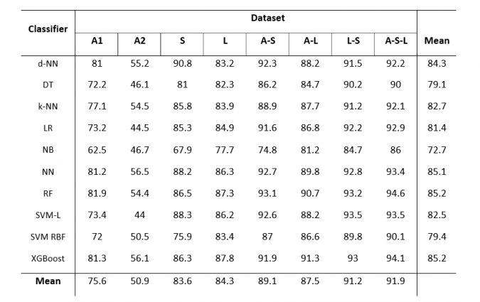
Machine learning has been widely used in remote sensing, with the commonly used machine learning algorithms being decision trees (DTs), random forest (RF), neural network (NN) and support vector machine (SVM). For this study, ten algorithms were used, namely random forest (RF), decision tree (DT), XGBoost, k-nearest neighbour (k-NN), naïve bayes (NB), logistic regression (LR), neural network (NN), deep neural network (d-NN), support vector machine (SVM) with linear kernel (SVM L) and SVM with radial basis function kernel (SVM RBF). A thousand data points were created using stratified random sampling and they were used as input for the algorithms, with 200 points assigned to each class (maize, cotton, groundnuts, orchards and non-agriculture). Each algorithm was cross-validated with a hundred iterations and each iteration was randomly split into a training dataset (70%) and test dataset (30%).

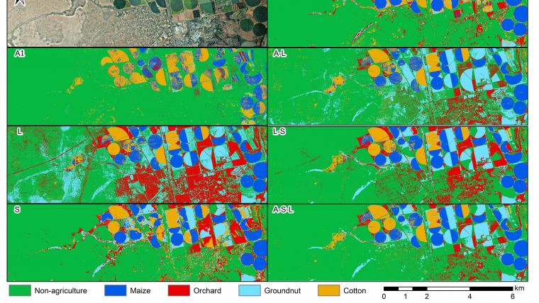
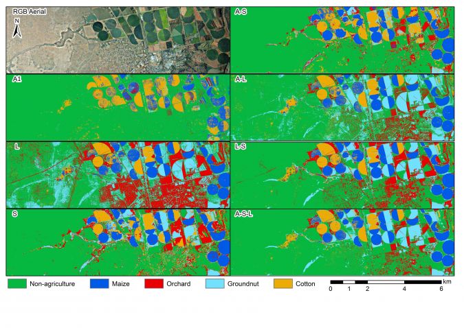
The results of the classification are summarized in Table 2, which shows the overall accuracy for the eight datasets and ten machine learning algorithms. Figure 2 shows a visual comparison of the random forest classification for seven of the eight datasets (A2 was excluded due to the low overall accuracies).

Discussion and conclusion

The machine learning algorithms were able to accurately classify the five classes by using the different dataset combinations as input, with nine of the ten algorithms obtaining at least one overall accuracy above 90% (random forest obtained the highest overall accuracy of 94.6%). The three main datasets (aerial imagery, Lidar and Sentinel-2) were able to obtain acceptable overall accuracies when used on their own, with the Lidar dataset and Sentinel-2 dataset obtaining similar overall accuracies. Although the Lidar and Sentinel-2 dataset performed on par with each other, the Sentinel-2 data has the advantage of being regularly updated (once every five days, depending on cloud cover), while Lidar data is typically updated less frequently. However, the Lidar data was able to differentiate between crop types on its own and proved to be particularly useful when distinguishing between different crops with noticeable height differences, such as orchards and groundnuts.

It is clear from the results that higher overall accuracies were obtained when the datasets were combined. The combination of all three datasets obtained the highest overall accuracies, although the combination of Lidar and Sentinel-2 performed just as well as the combination using all three datasets. Therefore, if available, Lidar data should be used in combination with spectral data in order to improve classification accuracies, especially for differentiating between crop types that have similar spectral signatures but clear structural differences (i.e. differences in height).