Lidar: Organising the Unorganised
A Lidar sensor generates hundreds of millions of XYZ coordinates in a few hours. From this massive number of sampled points one wants to reconstruct surfaces Lidar points are described as being ‘unorganised’; they form clouds. How to convert the unorganised into the organised Lidar has gained widespread recognition as the main source for the reconstruction of real-world surfaces. Its many applications include the creation of accurate Digital Elevation Models (DEM) and 3D-city models for planning purposes. It offers benefits for planning, design, inspection and maintenance of infrastructure. Dunes, beaches, dykes and floodplains can be captured accurately and with a high level of detail, enabling coastal-erosion modelling, monitoring and flood-risk management. The goal of surface reconstruction is to approximate geometry, topology and features of a surface using a finite set of sampled points. The result of a Lidar survey is a dense cloud of irregular, distributed 3D points characterised by XYZ coordinates associated with attributes such as intensity of return signal. The central issues when dealing with Lidar data concern archiving and management of the data, generation of output suitable for use within GIS and CAD software, filtering of data for reconstruction of bare-earth surfaces and features such as buildings and trees, and visualisation of the data. Regarding the latter, see the article "3D Visualisation of Lidar Data" The main focus here is on generation of GIS and CAD output.
Interpolation
Representation of elevation data within a GIS and CAD environment is carried out preferably in raster format, elevation values being stored in the cells of a 2D regular raster. The transformation of an irregular point-cloud into a regular raster requires interpolation: computation of elevation values for non-sampled terrain points from sampled points. Reconstruction of the continuous surface requires definition of a function that passes through the sampled points. An infinite number of functions will fulfil this constraint and, unfortunately, no simple rule exists for determining which is best suited to a given dataset. Additional conditions have thus to be defined, which has resulted in the development of a wealth of interpolation techniques. Some conditions are based on geostatistical concepts (kriging) and others on locality. The latter assumes a relationship between the elevation of each point and other points in the vicinity, up to a certain distance away. One of the most simple and available methods is ‘inverse distance-weighted interpolation’. This assumes an inverse relationship between elevations of neighbouring points and their distance: the greater the distance, the less the elevation of a sampled point will contribute to computation of the elevation of the non-sampled point. There are also conditions based on smoothness and tension (splines) or ad hoc functional forms. Selection of the method of interpolation is often based on experience, experiment and availability of algorithms in the GIS system. But it must be kept in mind that results produced by the various methods may differ considerably and appropriate selection is crucial; wrong information may lead to potentially wrong decisions and faulty simulation results.
Data Swaps
The hundreds of millions of points generated by each Lidar survey cause computational complications during interpolation since it is not possible to store all this data in the internal memory of even the most sophisticated computer. As a consequence the data has to remain on larger but significantly slower disks. Operational weakness arises from data swaps between disk and RAM rather than computation when processing such massive volumes of data. Many practical algorithms therefore perform ‘segmentation’, breaking down the point-cloud into a set of non-overlapping sub-clouds each containing a small number of sampled points. The points in each segment are then independently interpolated. Based on this principle a vast number of segmentation methods have been developed, including simple breakdowns and ones based on Voronoi diagrams. An algorithm that copes efficiently with data swapping minimises the times a disk is accessed and spectacularly reduces runtime. Researchers are still looking for algorithms that reduce data swaps. Agarwal and co-authors1, for example, recently developed a scalable approach based on quad-tree partitioning of data into a set of non-overlapping segments, going on to confront the performance of their own approach with that of commercially available software. They found their own method was able to process nearly 400 million points using less than 1GB of Ram, while QTModeler 4 from Applied Imagery, processing approximately 50 million points using 1GB of RAM, performed best of the other methods.

Value staying current with geomatics?
Stay on the map with our expertly curated newsletters.
We provide educational insights, industry updates, and inspiring stories to help you learn, grow, and reach your full potential in your field. Don't miss out - subscribe today and ensure you're always informed, educated, and inspired.
Choose your newsletter(s)