Road Maintenance with an MMS
Accurate and Detailed 3D Models Using Mobile Laser Scanning
A mobile mapping system (MMS) enables laser data and images of a road and its vicinity to be collected from a van or other moving platform. Here, the author describes data collection and accuracy assessment of a pilot carried out in Finland. It is demonstrated that MMS data processed with sophisticated software is well suited for road maintenance tasks as many parameters can be accurately calculated from the 3D model.
An MMS survey enables highly detailed mapping of roads and their direct surroundings with high accuracy and within a short period of time, while minimising nuisance to traffic and risks of accidents. To prove its aptness for road maintenance, a pilot was conducted aimed at assessing the accuracy of the 3D model, determining road damage and deformations and using the 3D model to design the renewal of the road surface. Furthermore, the MMS survey delivered essential input for the resurfacing machine.
Data Collection
A 22km-long, two-lane section of the National Road 6 (NR6) in south-east Finland was captured with a Trimble MX8 composed of two Riegl VQ-250 scanners, four cameras – one recording the road surface and three pointing forward – and an Applanix POS LV 520 for positioning purposes. The two lanes, which are mostly bordered by forest, were both captured, i.e. forth and back, with a speed of 50 to 70 km/h. For georeferencing purposes, ground control points (GCPs) were painted on both sides of three sections of the road at an interval of 50m and measured using Trimble R10 GNSS and DiNi Level instruments. The length of each section was 500-600m, so 74 GCPs were placed in total. Processing was done with Terrasolid's TerraScan, TerraMatch, TerraPhoto, and TerraModeler. These modules run on top of Bentley’s MicroStation.
Accuracy
A major source of errors is the blocking of GPS signals due to tunnels, buildings, trees, rocks or other obstructions near the road. These errors could be corrected using the GCPs and the overlap between the forth and back recordings. To determine the relation between the number and distribution of GCPs versus accuracy, the number of GCPs was systematically reduced from all to a spacing of 500m (Table 1).
|
|
Raw data |
All GCPs |
GCP spacing |
||
|
100m |
200m |
500m |
|||
|
Z average magnitude |
12.8 |
0.1 |
0.3 |
0.5 |
2.5 |
|
Z standard deviation |
|
0.1 |
0.5 |
0.7 |
1.9 |
|
XY average magnitude |
7.4 |
0.7 |
1.3 |
1.8 |
2.4 |
Table 1, Relationship between accuracy [cm] and spacing of GCPs.
A GCP spacing of 100 to 200 metres provides good accuracy, but with coarser spacing the accuracy diminishes quickly due to the non-linearity of the drift of the raw trajectory positioning. For high-accuracy work, the spacing should not exceed 50m for elevation and about 250m for planar coordinates. In addition, the elevation of the GCPs should be measured using a levelling instrument to obtain high accuracy.
Road Surface
After matching the overlap between the forth and back recordings, all non-road points were removed automatically. Orthoimagery with 1cm ground sample distance (GSD) was generated to support detection of road damage and previous repair work (Figure 1). Centre and edge lines and road edges were then digitised manually from the combined laser data and orthoimagery resulting in an accurate vector dataset. The centre and edge lines were used to create a surface model which enabled the extraction from the laser data of ruts and potholes with a depth of at least 2cm. The vertical distance between the heights of inner and outer edges of the pavement (super-elevation) was visualised by across-road arrows and the gradients of the slope (Figure 2). Figure 3 shows seven classes of local slope gradients: red indicates smaller than 1%, orange 1% to 2%, yellow 2% to 3%, yellow-green 3% to 4%, green 4% to 5%, blue-green 5% to 6% and blue larger than 6%. Areas with high gradients will disturb driving conditions but will also have quick water run-off, while the water will remain on flat areas for longer.
Road Repair
The survey revealed an urgent need for renewing the asphalt. Road-design software is not well equipped for processing massive point clouds. Therefore the original 3D model was thinned and used for creating a new design surface which was imported into a machine control system and used for resurfacing the road. In addition, the data allowed an accurate estimation of the amount of materials needed for the surface renewal activities.
Concluding Remarks
Future solutions may include line-of-sight analysis (Figure 4), calculation of road-surface roughness and cross sections, automatic vectorisation of paint markings and road break lines and detection of objects in the vicinity of the road.
Acknowledgement
Thanks are due to Kjell Tuominen and Arttu Soininen of Terrasolid Ltd, and Manu Marttinen of NCC Roads Ltd.
Further Reading
www.terrasolid.com/download/presentations/2012/mobile_accuracy_and_control.pdf
Figure Captions
Figure 1, Potholes, ruts and other deformations with a depth of at least 2cm are shown in blue.
Figure 2, Super-elevation: the blue line marks the location of the road section (bottom)
Figure 3, Centre and edge lines are shown in white and local slope gradients shown as classes.
Figure 4, Objects blocking sight (orange); red numbers indicate the distances to an obstruction for which a driver will be unable to stop in time when driving at a speed of 100km/h.

Value staying current with geomatics?
Stay on the map with our expertly curated newsletters.
We provide educational insights, industry updates, and inspiring stories to help you learn, grow, and reach your full potential in your field. Don't miss out - subscribe today and ensure you're always informed, educated, and inspired.
Choose your newsletter(s)