Point Clouds: Laser Scanning versus UAS Photogrammetry

Are photogrammetric point clouds superior to Lidar point clouds, or is it the other way around? To address this topic of ongoing debate, the authors of this article conducted a terrestrial laser scanning (TLS) survey together with an unmanned aerial system (UAS) photogrammetric survey of a gravel pit. Comparison revealed that TLS is superior when the highest level of detail is required. For larger surveying projects, however, RTK-enabled UAS photogrammetry provides sufficient levels of detail and accuracy as well as greater efficiency and improved surveyor safety.

In modern surveying, the numerous measurement methods can be divided into two broad categories: 1) on-site surveying using GNSS receivers, total stations or levels, and 2) remote sensing methods using either laser scanners (Lidar) or photogrammetry. TLS and UAS photogrammetry are popular for many projects. Accuracy, point density, acquisition time, processing time and costs are all important criteria for evaluating performance. A comparison of TLS and UAS photogrammetry on a single project cannot give decisive answers, because the choice depends on the needs of the professional and the characteristics of the project. Nevertheless, a comparison can help to indicate the relative strengths and weaknesses of TLS and UAS photogrammetry (Figure 1), which was the goal of this study.

Site details

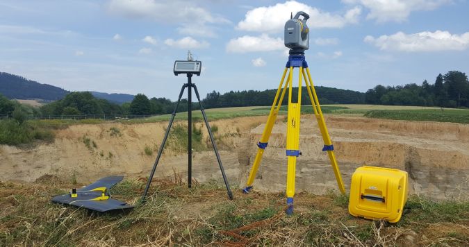
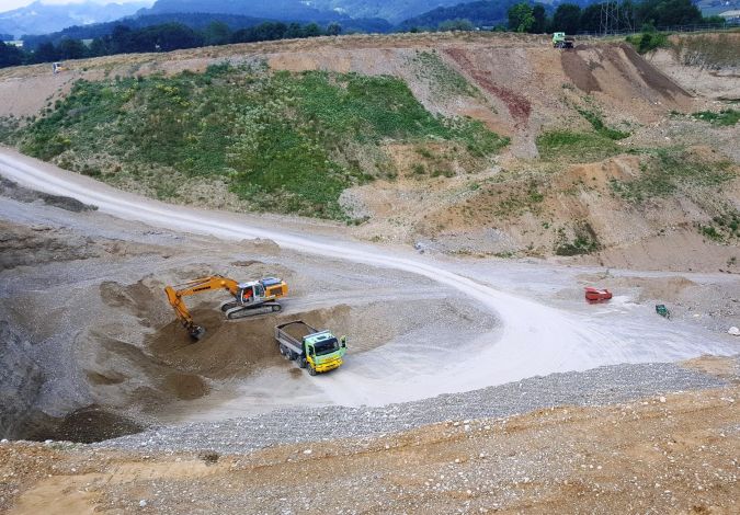
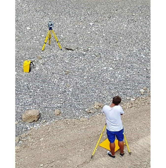
A four-hectare gravel pit in the Olten region of north-western Switzerland was chosen (Figure 2) as the site. For such sites, dense point clouds enable users to calculate slope and volume, detect toes and crests and generate contour lines. With a depth of approximately 40m, the gravel pit proved a challenge for UAS photogrammetry, due to the occluded areas resulting in interpolations and a decrease in accuracy. To georeference the TLS stations and to assess the accuracy of the UAS flights, nine ground control points (GCPs) were installed and their coordinates determined using a Trimble R10 GNSS receiver (Figure 3).

TLS Survey

The Trimble SX10 scanning total station was used to perform the TLS survey. Preparation for the survey involved determining the optimal distribution of GCPs and TLS stations. Each TLS station required line-of-sight to at least three GCPs, with these points distributed as evenly over the site as possible. To cover the entire site, three TLS stations were positioned outside the pit and two at the bottom of the pit. To orientate and set the position of the TLS, instrument levelling was required. A ‘free station’ method was then used to determine the 3D coordinates of the unknown station position with respect to the visible GCPs. On average, the TLS survey took 45 minutes per station, adding up to an on-site survey of nearly four hours.

UAS Survey

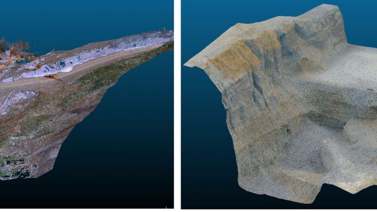
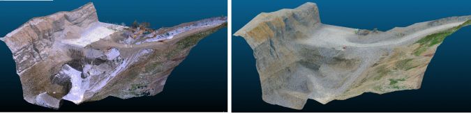
The UAS survey was carried out using a senseFly eBee Plus RTK/PPK. First, the route and flight boundaries were determined using eMotion 3, the eBee’s flight planning and management software. This professional software was used to outline the site, highlight the mapping area and generate flight paths automatically. To assess the influence of ground sampling distance (GSD) on the quality of the point cloud and define the optimum UAS workflow, flights were carried out at two heights: 100m and 150m. The eBee’s RTK capability was also used to receive RTK corrections and enhance the precision. This also helped to create four UAS point clouds. PC1 was captured at 100m, PC2 was captured at 150m, and PC3 was a merge of PC1 and PC2. PC1 and PC2 were georeferenced using GCPs. PC4 was captured at a flying height of 100m and georeferenced using RTK corrections only. A meadow next to the gravel pit was chosen as take-off and landing site. With Agisoft PhotoScan, digital surface models (DSMs) and an orthomosaic were generated. Figure 4 shows the TLS DSM and one of the UAS DSMs.

Performance Criteria

Performance criteria included on-site data collection time, in-office preparation time, data processing time and costs. With two UAS flights carried out at different heights and GCPs set across the site, the UAS point clouds could be compared on absolute accuracy and point density. Furthermore, it was considered whether RTK flight alone, i.e. without using GCPs, can give GCP levels of accuracy. Other factors investigated included the impact of flight height/GSD on point cloud quality and the effect on point density of the number of photos used in processing (the higher the flying height, the lower the number of photos).

Results

The georeferenced TLS point cloud and the four UAS point clouds were analysed in CloudCompare and Autodesk CAD Civil 3D; the results are listed in Table 1. UAS point cloud accuracy is at the level of a few centimetres, while TLS points have an accuracy of a few millimetres. In addition to this, TLS produces higher point densities than UAS images. As a result, the TLS point cloud was used as reference for comparison of the UAS point clouds. CloudCompare helped to assess the offset and standard deviation (σ) between two point clouds. AutoCAD was used to complete a volume comparison using the same base surface for all point clouds. Cut and fill volumes were then compared to this surface.

Table 1: Performance of four UAS point clouds using the TLS point cloud as reference; PC3 was generated by merging PC1 and PC2; ΔV: volume difference.

The UAS point cloud georeferenced with GCPs and the UAS point cloud georeferenced with RTK only both showed minimal offset and similar standard deviations with respect to the TLS reference. This indicates that ground control points are not required to ensure high absolute UAS accuracy (Table 2). The TLS point cloud has a very high point density, and while the UAS point clouds are less dense, they appear to show enough detail for most typical survey applications. The noise of the UAS point clouds was not assessed, but when compared against the TLS point cloud showed similar standard deviations and minimal offsets, indicating that the noise from UAS and TLS sources is irrelevant. All point clouds were perfectly exploitable, and the DSMs, volumes and other derived products were not affected.

Table 2: Comparison of performance criteria time including the time needed for on-site data acquisition and in-office processing.