Traffic Noise Mapping

Traffic is a common source of noise. Standards for noise pollution have been developed in many countries to safeguard human health and wellbeing. However, regulations may be inadequate in developing countries, where fast urbanisation, industrial growth and traffic increase create environments with hazardous noise levels. In India noise monitoring is done through actual measuring of sound levels at strategic locations. Continual measuring at many locations is, however, costly and unfeasible. Better to combine measurements with noise-propagation models. The authors developed such a method, and the resulting noise maps would seem sufficiently accurate.

The sound pressure at any location (receiver) is a function of all the sounds created in its neighbourhood (sources), the directions in which sounds are radiated from these and attenuation of sounds during propagation through the atmosphere above terrain. The farther from the source, the less the sound level; this is attenuation due to geometric spreading. Barriers such as buildings and walls also prevent direct transmission and thus reduce the level of sound pressure at the location of the receiver. The ground between source and receiver too contributes to or attenuates sound energy reaching the receiver. By adding together these three major sources of attenuation - geometric spreading, barriers and ground effects - one obtains the total attenuation. The sound level at a certain location is arrived at by adding the sound pressure level (SPL) of all sound sources to their directivity indexes and subtracting from this sum the total attenuation.

Data and Study Area
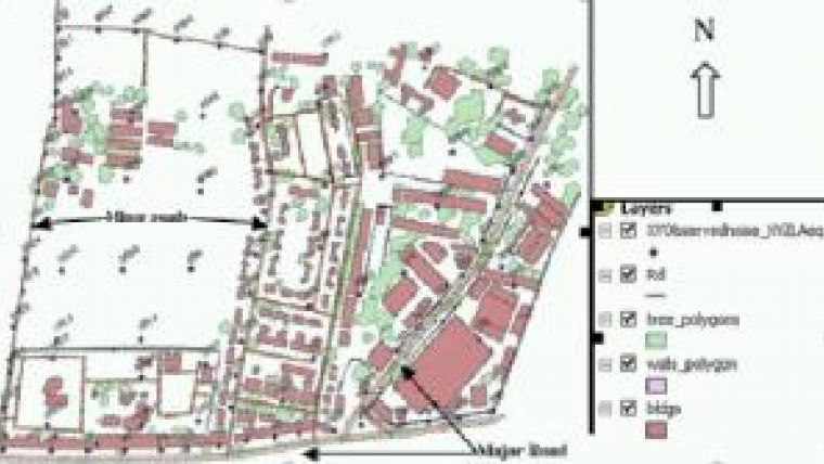
Modelling the sound pressure levels of traffic noise at any location in an urban area requires not only the availability of noise information, but also geo-information concerning roads and major sources of attenuation: buildings, walls and trees. High-resolution satellite images, easily procured or obtained for free via the internet, are well suited for digitising this type of geo-information. Figure 1 shows the map created for our study sample, a 0.33km2 area in Rawatpur, Kanpur, India, augmented with the location of reference points. To obtain the average building height in the study area the heights of individual buildings was estimated, though a better method would be based on the length of shadows. In Rawatpur sound levels are highest between 9:00 and 12:00, and over this time span sound measurements were conducted both at sound sources and at 56 locations well distributed over the urban area. The latter measurements are used as reference values for evaluation purposes. The sound generated by traffic on the road is actually a line source; we, however, model it as a sequence of point sources for purposes of ease of computation. Along the roads we measured sound pressure levels at 26 points to characterise the line sources, and at five locations to characterise point sources. The positions of sound sources and reference values were measured using GPS.

Good Results
Using the above model and data, sound pressure levels were predicted for the 56 reference locations within a GIS environment, taking into account buildings, walls, trees, and sound source characteristics. Figure 2 confronts the measured sound pressure levels with predicted values as computed for 34 reference locations using our method. The predicted noise at the reference location was computed from octave-band mid-frequencies from 63Hz to 8,000Hz, which takes into account the three major attenuations mentioned above. 

Interpolation was then carried out using Kriging, and a noise map created (Figure 3). Comparison with the map generated from sound-
pressure levels measured at the 56 reference locations (Figure 4, below) indicates that our method is good enough for community noise mapping, with a standard deviation of about 2dB (Table 1). Deviations may be due to incidental sources, such as barking dogs or music.

Table 1, Comparison of predicted and observed sound levels.

Concluding Remarks
Our method has the potential to replace or reduce the need for frequent measuring of sound-
pressure levels at many points in urban areas. The number of sound sources on which measurement has to be carried out, or the duration of measuring, can be reduced with better understanding of noise characteristics and improved planning of measurement locations. The present use of average building heights can be refined by taking into account the full three dimensions of individual buildings.

Acknowledgements
Thanks are due to Dr. Bharat Lohani, who leads the laser scanning research group at IIT Kanpur, India, and Manju Gupta, senior officer at Regional Office of UP Pollution Control Board at Kanpur.

Further Reading

• AEA Technology Rail BV, 2005, Harmonised Accurate and Reliable Methods for the EU Directive on the Assessment and Management Of Environmental Noise, Utrecht, www.imagineproject.org.
• Basic data sheet, District Kanpur Nagar (34), Uttar Pradesh (09), Source Census of India 2001, http://kanpurdehat.nic.in
• Bruel and Kjaer, Measuring Sound, www.bksv.com
• Noise standards, Noise Pollution (Regulation and Control) Rues, 2000, www.cpcb.nic.in/Noise_Standards.php
• Noise monitoring data, Central Pollution Control Board, India, 2007, www.cpcb.nic.in/Noise_Monitoring_Data.php