UAV Spectral Image Mapping of Shoreline Vegetation

An affordable DJI Phantom 3 drone with built-in camera, which collects data only in the visible spectral bands, has been used to identify shoreline, vegetation and water.

Rapid identification of a clear water surface, shoreline and vegetation can serve as a means of water-level monitoring and as an important indicator of changes. In cases when a high level of detail or on-demand data collection is required, unmanned aerial vehicles (UAVs or ‘drones’) can provide a good service. It is important to think about the costs of the UAV and the connected sensors as well. Multispectral and thermal cameras are still very expensive in comparison to visible cameras. This article shows how a commercially available middle-class drone (DJI Phantom 3 with built-in camera), which collects data only in the visible spectral bands and is affordable even for individuals, can be easily used to calculate colour spectral indices to identify shoreline, vegetation and water.

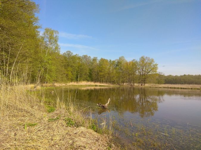
An area lying to the north of the city of Pardubice in the Czech Republic is very rich in ponds. The area of interest is flat, lying approximately 220 metres above sea level. It comprises clear water surfaces, seasonally flooded greenery, vegetation including treetops, dry reeds (including dry grass) and dry trees (see Figure 1).

Flight Planning and Data Collection

The dataset was captured on 20 April 2018, i.e. in spring. The flight was planned in advance in DJI GO and then sent to the drone. The drone automatically flew according to the plan. It took approximately 15 minutes to cover the area of 0.0285km² so no break in the flight was necessary. The total length of the flight was 1,545m, and it was planned in seven main lines consisting of 64 waypoints in total. Front and side overlap were both 60%. Average speed was 2.2m/s, altitude was 39.6m and resolution was 1.7cm per pixel.

Data Processing to Calculate Vegetation Indices

Two software tools were used: Pix4Dmapper 4.2.27 trial and ArcGIS for Desktop 10.5.1. Pix4Dmapper was used for a mosaic building and calculating all indices. ArcGIS was used for visualisation of the resulting indices. WGS 84 – UTM zone 33N was used as a coordinate system.

The final mosaic was created from 33 images, covering 0.012km². Certain types of land cover require a higher overlap, so images showing only treetops were not aligned because of the lack of common points. Nevertheless, the final mosaic covered the whole shoreline so it was perfectly usable for the next step.

The survey team calculated various colour-based vegetation indices, which are based only on red, green and blue bands: CIVE, ExG, ExR, GRVI, NDI, TGI, VARI and VDVI. Several colour band combinations and combinations of particular indices were calculated as well to include different approaches described in the literature.

ArcGIS was used for visualisation of the results because it provides more visualisation methods and better tools for map creation. The “Pink to YellowGreen Diverging, Bright” colour ramp was used for all indices, which helped to visually distinguish between particular land cover types. The other settings were: stretched visualisation, percent clip stretch (both min. and max. 0.5). Green colour represents the highest values, dark pink represents the lowest values, and yellow represents medium values in all cases to simplify comparison of the results. An inverted scale would be more natural in some cases, e.g. for displaying vegetation with the green colour.

Results and Interpretation

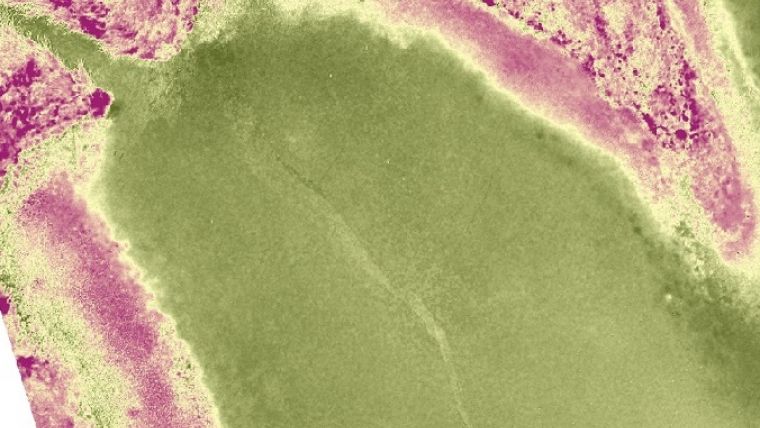
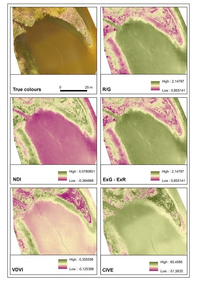
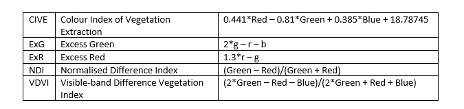
Based on the visual interpretation and literature, the following colour indices were chosen as the most suitable ones: CIVE, ExG – ExR, NDI, Red/Green ratio and VDVI (see Figure 2 for results and Figure 3 for calculating algorithms).

The clear water surface is highlighted by R/G, ExG – ExR (dark green in both cases) and NDI (dark pink). The water surface can be easily distinguished from the seasonally flooded greenery. The borderline between the clear water surface and seasonally flooded greenery is indiciated by the yellow line. Green vegetation is highlighted by all indices. VDVI and CIVE clearly highlight treetops, displaying green and dry vegetation in dark colours so that these two types of land cover can be easily distinguished. Seasonally flooded greenery is well visible with R/G, NDI, ExG – ExR and VDVI because it is bordered by a yellow line. The best result is provided by VDVI (green colour).  Dry reeds and dry trees are well highlighted by VDVI (dark pink) and CIVE (dark green).

Comments on the Indices

VDVI is very useful for differentiating green vegetation from dry vegetation. R/G (and its opposite G/R) makes it easy to distinguish between vegetation and the clear water surface. The ExG – ExR difference makes it possible to distinguish all vegetation from the clear water surface. NDI makes it possible to distinguish all vegetation from the clear water surface. CIVE clearly highlights green vegetation, which can be easily distinguished from dry vegetation (both trees and reeds). The clear water surface cannot be easily distinguished because it is visualised in a similar way as dry vegetation.

Conclusion

Shoreline, vegetation and the clear water surface can be easily monitored by a middle-class UAV equipped with a camera recording only in the visible spectral bands. It provides data with a very high spatial resolution on demand and at acceptable costs. It can significantly help with monitoring of less accessible areas such as overgrown or waterlogged terrain, as in this case. Particular land cover types can be easily distinguished by a visual interpretation as the first step. Vegetation indices based on visible spectral bands appropriately complement the visual interpretation. They can quickly highlight vegetation, seasonally flooded vegetation and the clear water surface to enable identification of the shoreline as well. Each index emphasises different types of land cover so it is beneficial to combine multiple indices.

Acknowledgement

This research was supported by the University of Pardubice, Project SGS_2018_19.

Further Reading

Hamuda, E., Glavin, M., Jones, E. (2016) A survey of image processing techniques for plant extraction and segmentation in the field. Computers and Electronics in Agriculture 125(C), pp. 184–199.

Meyer, G.E., Neto, J.C. (2008) Verification of color vegetation indices for automated crop imaging applications. Computers and Electronics in Agriculture 63(2), pp. 282–293.

Ponti, M.P. (2013) Segmentation of Low-cost Remote Sensing Images Combining Vegetation Indices and Mean Shift. IEEE Geoscience and Remote Sensing Letters 10(1), pp. 67-70.