Constructing Very High Resolution Satellite Data Surface Models

A digital surface model (DSM) is a common photogrammetric product which is widely applied in the areas of surveying and mapping as well as geographic information systems (GIS). In line with the invention of the semi-global matching (SGM) algorithm by H. Hirschmüller in 2005, stereo pairs are matched pixel-wise, leading to a very dense DSM. Very high resolution satellite (VHRS) imaging sensors provide stereo images at up to 0.3m ground sampling distance (GSD). The major advantage of VHRS data is that the data coverage is much larger than that of classical airborne data. Therefore VHRS imagery is a promising option to generate 3D point clouds and DSMs. A recent study compared it with the ISPRS Lidar benchmark data.

To verify VHRS algorithms, a VHRS benchmark dataset of an area in Catalonia (Spain) is provided by the ISPRS Working Group I/4 on Geometric and Radiometric Modelling of Optical Spaceborne Sensors. The data for the benchmark was laser scanned by the Institut Cartografic de Catalunya (ICC) and functions as a reference dataset.

The University of Stuttgart – Institute for Photogrammetry applied a Worldview-1 (WV-1) dataset at 0.5m GSD to the ISPRS benchmark using their own processing algorithms. The data was acquired on 29 August 2008, with a stereo angle of the pair of 35 . The dataset contains three different regions: La Mola, Terrassa and Canarisses. For each region, the size of the stereo image is approximately 8,000 x 8,000 pixels. These regions cover rural, urban, forest, flat and mountainous areas. All the data is delivered at Level 1B, which provides radiometrically corrected imagery in top-of-atmosphere (TOA) radiance values and in sensor geometry. The data contains the corresponding rational polynomial coefficient (RPC) files, which describe the exterior orientation of the satellite orbits.

Processing VHRS data

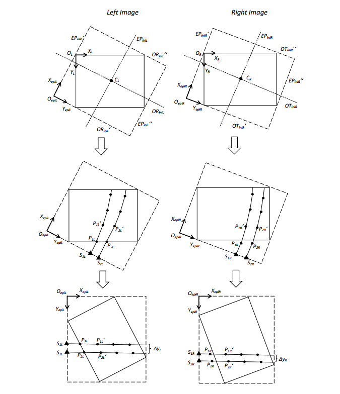
The algorithms used were implemented as an automatic pipeline to generate both point clouds and DSMs. Normally the first procedure is the RPC-based bundle block adjustment but, because the orientation of the benchmark dataset’s RPC files were already available, the actual first step was epipolar resampling. In epipolar resampling, corresponding points are located on the same row in the file so that the calculating time and memory usage is reduced. In a standard aerial camera geometry, the epipolar points are all on a straight line. However, in a VHRS image they are more like hyperbolas.

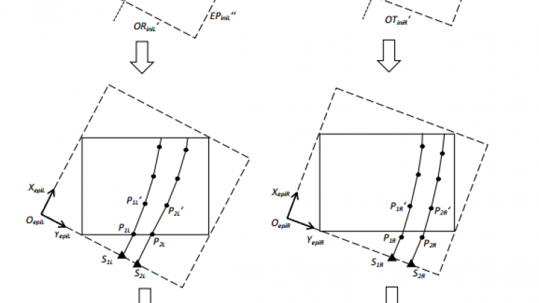
To approximate the hyperbola, a modified piecewise epipolar resampling method based on J. Oh’s research was used (Figure 1). In this resampling method, a number of steps are performed. The first step is to define the coordinate system of the stereo epipolar image. The centre point of the left image is used to calculate the direction of the initial epipolar curve and its orthogonal line. The next step is the determination of the start point for the epipolar curve pair generation from the bottom boundary of the left image. According to the characteristic of a VHRS image’s epipolar curve, the local epipolar curves are approximated using the projection-trajectory method. For the epipolar segment inside the image, a pre-defined length of the segment is given and a new epipolar segment will be generated if it reaches the pre-defined length. In the last step, the stereo images are resampled along the epipolar segments.

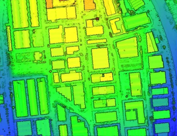
The dense image matching is now based on the resampled epipolar stereo pair. The C/C++ library LibTsgm is applied and integrated in the processing pipeline for pixel-by-pixel matching. LibTsgm implements a modified SGM method and was developed at the University of Stuttgart – Institute for Photogrammetry and then outsourced to nFrames GmbH in Stuttgart in 2013. When the dense image matching is finished, 3D point clouds are calculated; from these point clouds, the DSMs are generated with a GSD of 1m. For better visualisation, the point clouds are meshed by CloudCompare (Figure 2).

Point cloud accuracy

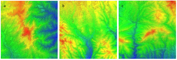
In order to investigate the performance of the 3D reconstruction pipeline, three different types of terrain (samples) have been extracted from the point cloud to show more detail (Figure 3): a) mountainous forest area, b) flat rural area, and c) urban area. The point cloud from the VHRS data is in general coarser than that of the reference Lidar point cloud. The extracted DSMs are compared with the reference Lidar point clouds. The height between the processed WV-1 DSM and the Lidar point cloud is compared and, from this comparison, difference charts are created.

The basic terrain of the mountainous forests is reconstructed well in the satellite data, with most height differences less than 2.5m. In the flat rural area, some detailed features are missing in the VHRS point cloud but overall height differences are at the sub-metre level. In the urban area, the buildings in the Lidar point cloud have sharper edges than in the VHRS data and most details are missing, although the WV-1’s point cloud can reconstruct some details on the roofs. Most height differences are less than 2m in urban areas.

A further investigation of the accuracy shows that overall accuracy is affected by shadows in the scenery. As a result, the accuracy in the flat rural area is the best as there are minimal shadows. The buildings create many shadows that influence their reconstruction and affect the accuracy. The accuracy of the mountainous forest area is affected by the shadow of the trees as well as the steep height changes.

DSM accuracy

The Lidar point cloud is processed into a reference DSM in order to compare the DSM from the VHRS. To evaluate the accuracy of the 3D reconstruction, the root mean square error (RMSE) has been calculated according to the height differences of the DSMs. This shows that the RMSE of the La Mola test site is about 3.1m, of the Terrassa test site is 2.8m and of the Canarisses test site is 3.4m. The Terrassa test site has a better RMSE because it has more flat areas.

For a robust estimation, the normalised median deviation (NMAD) between the two DSMs is calculated. The corresponding 68% and 95% quantiles of absolute errors are also taken. The distributions of the height differences are depicted as a histogram for each test site. The NMAD varies between 0.8 and 1.4m with the 68% varying between 1.4 and 1.9m and the 95% varying between 7.0 and 8.3m (Table 1).

Table 1, Overview of DSM comparison.

Conclusion

The automatic 3D reconstruction pipeline of the (V)HRS data has been verified as an accurate and robust method. The generated 3D point clouds and DSMs are very dense, and the main texture information of the test sites is reconstructed. The DSM has some outliers and the edges of buildings are not sharp because of the influence of shadows and low image redundancy. Better results could possibly be obtained if higher resolution data (e.g. 0.3m GSD satellite imagery) and multi-view imagery are applied in future work.